2 Getting Started
This chapter will help get you up to speed using both R and RStudio. However, to do so we will need to simultaneously introduce a large number of concepts. Don’t worry if you don’t pick up on all of them right away! We will necessarily need to do a deeper dive into each throughout the book.
After reading these notes you should be able to:
- Run R code interactively.
- Use keyboard shortcuts in RStudio.
- Perform basic mathematical calculations using R.
2.1 Using R
There are many ways to use R, that is to run code written in the R programming language.
2.1.1 Batch Mode
One way to run R code is in batch mode. Suppose we had a file named some-script.R which contained the following code:
# create some random data
some_data = data.frame(
  x = rnorm(100),
  y = rnorm(100)
)

# write this data to a file
write.csv(some_data, file = "some-data.csv")
To run this code, which we often call a script1, we would type Rscript some-script.R in a terminal window followed by the name of the script we would like to run.
user@machine:~$ Rscript some-script.RAlternatively2 we could use:
user@machine:~$ R CMD BATCH some-script.RIn either case, the code in the script some-script.R would be run as R code and the result would be a file written to disk. As the user, we would not see any of this happening. You could think of this as running R code as a background process. The only noticeable effect of this script would be the file that the script created.3
While this is incredibly useful, especially for more general purpose programming, for the most part this will not be how we use R.
2.1.2 Interactive Mode
When using R for data tasks, especially data analysis, it is often most useful to use R in interactive mode. For our purposes, that is helping you learn R, this will be particularly useful as it will allow us to see what R is “doing” when we run code.
To run R in interactive mode, simply type R in a terminal.4
user@machine:~$ RAs a result, you will see something like the following:
R version 4.2.3 (2023-03-15) -- "Shortstop Beagle"
Copyright (C) 2023 The R Foundation for Statistical Computing
Platform: x86_64-pc-linux-gnu (64-bit)

R is free software and comes with ABSOLUTELY NO WARRANTY.
You are welcome to redistribute it under certain conditions.
Type 'license()' or 'licence()' for distribution details.

R is a collaborative project with many contributors.
Type 'contributors()' for more information and
'citation()' on how to cite R or R packages in publications.

Type 'demo()' for some demos, 'help()' for on-line help, or
'help.start()' for an HTML browser interface to help.
Type 'q()' to quit R.

>
We now have access to a read–eval–print loop, which is often simply called a REPL.
- Read: The user’s input will be collected. Your input will essentially be the code you write.
- Eval: The code you supply will be evaluated. We often call this “running” or “executing” your code.
- Print: The result of evaluating your code will be printed, so that you can see the effect your code had.5
The > at the very end is a prompt suggesting that you can now input R code. Typing R code and pressing Enter will evaluate code. This is something we will do, however, we would like some way to both keep track of what code we run, and more importantly, compose it before we run it. To accomplish this, we will need a text editor or an IDE.
2.2 Using RStudio
RStudio is a free and open-source integrated development environment (IDE) for R, but what does that mean? Most importantly, it simultaneously provides access to a text editor (where you will write code) and an R interactive session (where you will run code), with a number of features linking the two. More specifically, RStudio provides:
- A text editor6 that has many features that will specifically assist with writing code in many languages, but in particular R code.
- An interactive R session (a REPL) which is running in a window called the console.
- In newer versions of RStudio7, and depending on your operating system, access to a terminal, which would allow for, among other things, running R in batch mode.
- The jobs panel assists in creating and running batch jobs.
- An environment viewer which will help you track objects you have created in interactive sessions.
- A file manger that allows you to view, open, and manages files.
- A plot viewer which will allow for quick previewing of any graphics generated in an interactive R session.
- A packages viewer which will help manage installed R packages.
- A help panel that will display relevant R documentation.
These items (and more) are arranged into four different panels, each with tabs that contains a specific element.8
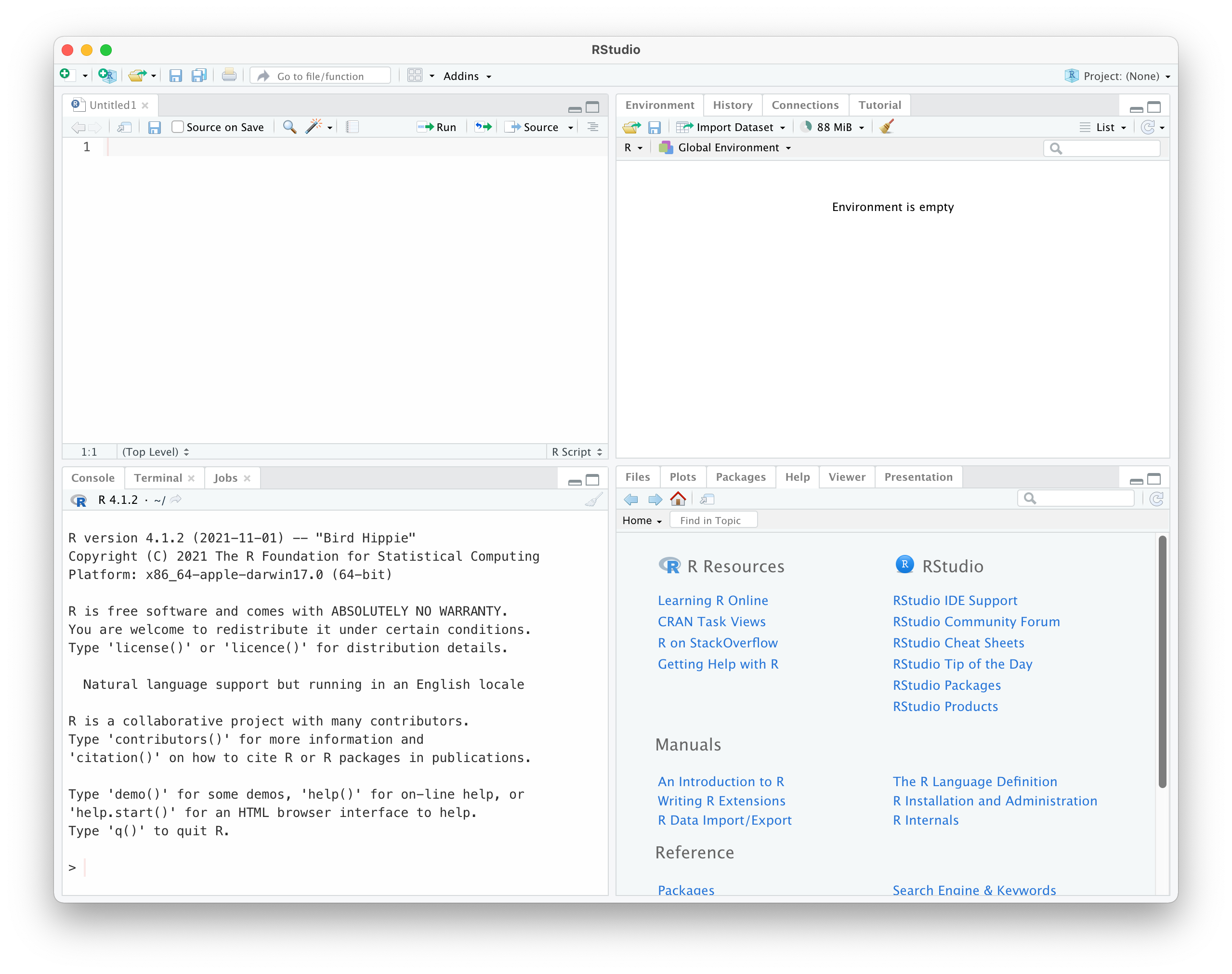
The specific arrangement of these panels can be modified by RStudio’s preferences, but as you can see, they are always labeled so that you can find them.
2.3 Writing Code
It may seem like a good idea to type directly into the console as you can then immediately run the code by pressing Enter on your keyboard. However, this is a bad habit for a number of reasons. It is sometimes appropriate, and later we will emphasize when that is, but to start, we recommend typing all of your code into an R script. To create a new R script, you could use the RStudio menus and select File > New File > R Script. Do not do this. Instead, use the appropriate keyboard shortcut, which is also displayed in the previously mentioned menu. For quick reference:
- macOS: ⌘ + ⇧ + N (
Cmd+Shift+N) - Windows:
Ctrl+Shift+N - Linux: We trust that you can figure it out.
This will open a new R script where you will type commands that we will run in these notes.
2.4 Running Code
Suppose you now have an R script open, and you’ve typed some code. There are generally two approaches you will take:
- Run the code line-by-line based on your cursor placement.
- Run a selection of the code.
Copy-paste9 the following code into a blank script:
2 + 2
3 - 4
5 * 2
4 / 2
After doing so, place your cursor on the first line. To run this line of code, you could click the Run button in the text editor. Do not do this. Instead, use your mouse to hover over this button. By doing so, it will reveal the keyboard shortcut for this action for your specific operating system.
- macOS: ⌘ + ↵ (
Cmd+Enter) - Windows:
Ctrl+Enter - Linux: We trust that you can figure it out.
Try using this both by first placing your cursor on a particular line, or also by first highlighting one or more lines. Notice that the results of running code are visible in the console tab.
2.5 Mathematical Calculations
Now that we can write and run code, we can try out R by effectively using it as a replacement for a simple calculator.10 Before doing so, a few notes about order of operations.
2.5.1 Operator Precedence
What is the result of evaluating the following mathematical expression?
\[ 18 \div 2 - 3 \times 3 \]
You probably guessed \(0\). And you’d probably suggest it would be wrong for someone to guess \(18\). What if I told you both can be right? Actually, that is what I’m telling you, because it is true, depending on how you define the order of operations which in programming terminology we would call operator precedence.
Yes, there is a generally accepted order of operations that we’re all aware of, and R generally matches this, but it is important to be aware of these rules, especially because in addition to the mathematical operators that you are already familiar with, R will introduce a number of additional operators for which you will need to understand their place in the precedence ordering.
For an exhaustive list of this ordering, run the following code11:
?SyntaxThis will bring up the R documentation, in the Help tab in RStudio, which clearly defines operator precedence in R. You are not expected to memorize this. What you are expected to do is know that operator precedence exists, and importantly, that you can always simply reference this document to refresh your memory on operators that you do not frequently use.
Like mathematics, parentheses should be used liberally to create groupings that make it easier for a reader to parse your expressions.
\[ (18 \div 2) - (3 \times 3) \]
Notice how the following two R expressions both evaluate to 0, but at a glance, it is much easier to parse the meaning of the second example.
18 / 2 - 3 * 3#> [1] 0(18 / 2) - (3 * 3)#> [1] 0Parentheses are your friends. Don’t be lazy. Use them.12
2.5.2 Arithmetic
R has the usual arithmetic operators, as well as a few your might not expect. Two of then, in particular + and - have both a unary (operates on a single object) and binary (operates on two objects) versions. For full documentation, run the following:
?ArithmeticUnary + is almost never seen, but unary - has an obvious and frequent use, that is, creating a negative number:
42#> [1] 42-42#> [1] -42When using a unary operator, you should not put a space between it and the object it operates on.13
R has the following binary operators which you are likely already familiar with:
- Addition:
+ - Subtraction:
- - Multiplication:
* - Division:
/ - Exponentiation:
^
Examples of each are given:
1 + 6 # addition#> [1] 72 - 5 # subtraction#> [1] -33 * 4 # multiplication#> [1] 124 / 3 # division#> [1] 1.3333335 ^ 2 # exponentiation#> [1] 25We can mix these together as we saw above, and in doing so they will follow the usual operator precedence for arithmetic operations.
18 / 2 - 3 * 3#> [1] 0But again, it is good practice to use parentheses to make your intent as clear as possible.
(18 / 2) - (3 * 3)#> [1] 0However note that, unlike written mathematics, parentheses do not create an implied multiplication. That is, something like the following will cause a syntax error.14
3(4 + 5)#> Error in eval(expr, envir, enclos): attempt to apply non-functionYou will need to explicitly request a multiplication.
3 * (4 + 5)#> [1] 27Two additional binary operators exist that you might not be familiar with that are more often used in programming than everyday mathematics.
- Modular arithmetic:
%% - Integer division:
%/%
The following is an example of modular arithmetic:
7 %% 5#> [1] 2The easiest way to think of the result is the “remainder” when attempting to divide, in this case, 7 by 5. This operator is often called the modulus operator and we would read this expression as “7 mod 5.”
Run these examples to get a better idea of how this works:
3 %% 5
5 %% 2 # this example in particular
4 %% 4
5.5 %% 3
The following are examples of integer division:
3 %/% 5#> [1] 05 %/% 2#> [1] 24 %/% 4#> [1] 15.1 %/% 3#> [1] 15.9 %/% 3#> [1] 1Hopefully it is clear that these return only the integer part of the division, where the decimal part is simply removed, not rounded.
Both the modulus operator and integer division can use a non-integer on the right-hand side, but this should likely be avoided.
Two additional mathematical operations that are available are a square root and absolute value function. For documentation, use:
?sqrtThey both behave as you would expect:
sqrt(9)#> [1] 3sqrt(22)#> [1] 4.690416abs(42)#> [1] 42abs(-4.2)#> [1] 4.22.5.3 Logarithmic Functions
Logarithms are extremely important in mathematics, and as such, R has a number of functions for working with both logarithms and their inverse, the exponential function.
Whenever you hear “logarithm” you should assume this means the natural logarithm, unless specified otherwise. Make this assumption even if it is written as \(\log\) and not \(\ln\) as you might have seen previously. The log() function in R is a so called natural logarithm by default.
The notion that \(\log\) without any qualifier could be considered a base 10 logarithm is a bad habit. When speaking with mathematicians or statisticians, they are almost exclusively using natural logarithms so they won’t bother to qualify what they mean by \(\log\) and you should assume they mean natural logarithm.15
For documentation of these functions, use:
?logFirst, some examples of the logarithm functions:
log(10)#> [1] 2.302585log(10, base = 10)#> [1] 1log(8, base = 2)#> [1] 3log10(100)#> [1] 2log2(256)#> [1] 8There is no ln() function in R. The log() function calculates a natural logarithm by default. It can be modified to calculate a logarithm with any base by using the base argument to the function. The log10() and log2() functions are shortcuts for logarithm base 10 and logarithm base 2 respectively.
Next, some examples of using the exponential function.
exp(1)#> [1] 2.718282exp(2)#> [1] 7.389056Note, there is no pre-defined constant e in R. To use the mathematical constant \(e\) in R, use exp(1).
Lastly we verify that log() and exp() are inverses of each other, as expected.
log(exp(1))#> [1] 1exp(log(1))#> [1] 1log(exp(42))#> [1] 42exp(log(42))#> [1] 422.5.4 Trigonometric Functions
R has many built-in trigonometric functions. For documentation of these functions, use:
?TrigR does have a built-in constant pi which represents the mathematical constant \(\pi\).
A few examples:
sin(0)#> [1] 0cos(0)#> [1] 1tan(0)#> [1] 0sin(pi)#> [1] 1.224647e-16cos(pi)#> [1] -1tan(pi)#> [1] -1.224647e-16You might have expected examples like sin(pi) to produce 0 as its result. Unfortunately, because of the way computers store numbers and perform mathematical operations, sometimes you will get odd results like this where instead of \(0\) you will get some very small but nonzero number. This is a consequence of floating-point arithmetic which is necessary because computers have finite memory, thus cannot perfectly represent irrational numbers like \(\pi\).16 More on this later when we dig into data types in R.
The trigonometric functions in R use radians, not degrees.
2.5.5 Special Mathematical Functions
R also contains the ability to use several so-called special mathematical functions. For documentation, use:
?SpecialThese functions are most often used in mathematical statistics contexts, so we will not see much use of them. Examples of two of the more common functions:
factorial(6)#> [1] 720choose(n = 10, k = 2)#> [1] 452.5.6 Rounding
R provides a number of functions for performing rounding type functionality. For documentation, use:
?roundThe ceiling() function will always round up, no matter the decimal part of the number.
ceiling(3)#> [1] 3ceiling(3.1)#> [1] 4ceiling(3.9)#> [1] 4The floor() function does the opposite, always rounding down.
floor(3)#> [1] 3floor(3.1)#> [1] 3floor(3.9)#> [1] 3The trunc() function truncates a number, that is, removes the decimal part of the number.17
trunc(3)#> [1] 3trunc(3.1)#> [1] 3trunc(3.9)#> [1] 3The round() function does what the name suggests and rounds its input.
round(pi)#> [1] 3round(4.2)#> [1] 4round(5.9)#> [1] 6By default it rounds to the nearest integer, but we could also round to a certain number of digits. For example:
round(pi, digits = 4)#> [1] 3.1416Similarly, we could specify a certain number of significant digits using the signif() function.
signif(123456789, digits = 4)#> [1] 123500000Notice that this returns the original number rounded to the requested number of significant digits.
However, be aware that the round() function has one interesting behavior you might not anticipate.
round(4.5)#> [1] 4Use ?round to access the documentation. Read the details about “round to even” which explain this anomaly.
You can express numbers in R using scientific notation. Additionally, R will sometimes return results using scientific notation. Some examples:
10e3#> [1] 100001.23e-4#> [1] 0.000123There is an internal R option that controls when R reports results using scientific notation, but it generally does so for very large or very small numbers.18
100000000000#> [1] 1e+110.000000000006#> [1] 6e-12Beware of floating-point arithmetic oddities when using these functions. The weird behavior of round() can be attributed to the realities of doing arithmetic using a computer. Floating-point arithmetic will be a running theme causing things to not work exactly as expected.
2.7 Documentation
Several times throughout this chapter, we have referenced the R documentation. To access the documentation for a particular function, use ?name_of_that_function. Alternatively, instead of the ? operator, you could use the help() function. For example, help(log). To access documentation on a particular operator, like +, surround it by backticks, ?`+`.
Documentation will be something that we return to several times. Right now, much of the documentation will be difficult to decipher. As you learn more about objects and functions in R, we’ll return to a discussion about how to best read R documentation.
2.8 Summary
In this chapter you’ve learned to use R for simple mathematical calculations, but this is just the very beginning of what R is capable of. Don’t worry if you didn’t catch all of the minor details, that is what the rest of this book is for!
2.9 What’s Next?
In the next chapter chapters we will:
- Investigate objects and functions!
- Give a hint as to why output often begins with
[1], which is related to the lack of scalars in R.
We use script and program somewhat interchangeably.↩︎
These days, using
Rscriptis likely preferred over usingR CMD BATCH. We mostly showR CMD BATCHas a means to illustrate why this is called batch mode. However, if you find yourself needing to run R in batch mode, consider the excellentlittlerpackage.↩︎Had we not specifically written code to create a file, there would be no noticeable effect whatsoever!↩︎
You can also obtain an R interactive session by running a program called R GUI if that was provided with your R installation. You probably do not want to do this as RStudio will provide all the same features, plus many more, all in a much easier to use package.↩︎
Later we will stress that what is printed is not what is returned. What is printed is R doing the best job it can to represent the computer objects you create in a human readable or interpretable manner.↩︎
Choice of text editor is a hotly contested topic among seasoned programmers. There will always be an argument as to which of
vimoremacsis better. If you’re already avimuser, note that RStudio allows you to usevimbindings. If you’re anemacsuser, consider looking into Emacs Speaks Statistics. If you don’t know what either of these are, which we assume is the case for most readers, we highly recommend using the built-in RStudio text editor. Do not use Notepad on Windows. Do not use Microsoft Word. Do not use a Google Doc. None of these have features that are helpful for coding, and some have features that are detrimental.↩︎You’re running an up-to-date version of RStudio, right?↩︎
When you first open RStudio, you will only see three of the four panels. The fourth appears when you open or create a file to be edited.↩︎
You used a keyboard shortcut, right?↩︎
Hopefully, after learning to appreciate R, or scientific computing in general, you will never again reach for a calculator other than R unless an instructor requires you do so for an exam.↩︎
This is a great example of code that you do not need to enter into a script first, as there really isn’t a need to maintain a record of it. Simply copy-paste this directly into the console.↩︎
The documentation and reference manuals are somewhat ambiguous as to where
(falls in the operator precedence list. When in doubt assume it is the highest order precedence. That is, evaluate things within the (deepest set of) parentheses first (following operator precedence in doing so) then apply operator precedence as usual. In many ways, parentheses act more like a function than an operator. For additional details, see the Parser chapter of the R Language Definition or the Parsing and Grammer section of Advanced R. Note that both of these sources are well beyond the scope and level of these notes.↩︎This is a note about code style which we will give a more complete explanation of later. In short, code style is concerned with how the code looks even though code that looks different sometimes is evaluated the same way. In this case, with or without the space, that is
- 42or-42, the code will perform the same operation. Run both yourself to verify this.↩︎The particular error here suggests that it looks like your are trying to use a non-function as a function. This will become more obvious when we discussion function syntax in detail.↩︎
This is likely true for computer scientists as well, but they also have good reason to use base 2 logarithms.↩︎
This article from the Jet Propulsion Laboratory (JPL) will offer some insight as to why this is not an issue: How Many Decimals of Pi Do We Really Need?.↩︎
The difference between
floor()andtrunc()is very subtle. Read the documentation to learn more.↩︎It is not recommended that you alter this setting.↩︎
This symbol goes by many names, but it is absolutely not a hashtag because with only the symbol, there is no tag. You might also hear this symbol referred to as a number sign or pound sign.↩︎
Other programmers often also includes your future self.↩︎
Stylistically, we expect to see a space before a
#if is used on the same line as code. Nothing should precede the#if it is on its own line. Also put a space after any#. Again, these are subjective stylistic choices, but they will be used throughout these notes.↩︎
2.6 Comments
Throughout this chapter we have used code comments without any explanation. In R, comments are defined using a hash,
#.19Comments in code are essentially human readable notes to other programmers.20 They are ignored when the computer evaluates the code.
Note that comments can be on their own line, or a the end of a line that also contains code. Note that neither of the above comments had an effect on the output.21
It is more of an art than a science when it comes to knowing when and where to write comments. Comments should help a reader understand what your code does. It should not simply state exactly what the code does, line-by-line, but instead be a more abstract human interpretable explanation. As beginners, error on the side of more comments than less.